Chapter 3: More Measures of Central Tendency and Spread: Mean, Standard Deviation, Z-scores
Chapter 2 focused on a measure of central tendency (median) and spread (the distribution and variation of data variation, through 5 point summaries and box plots). Chapter 3 focuses on another measure of central tendency: mean, and another measure of spread: standard deviation.
Statistics in Action
In order to show you how mean and standard deviation operates at different levels of measurement, this chapter will have examples around three questions. We will explore, within a U.S. context, (gender and racial) pay gaps, feelings towards journalists following the 2020 election, and Christian proselytization.
1. Mean
Definition: Mean
Mean: The averagea value; the value each case would have if all cases’ values were redistributed equal among all the cases.
a While both the mean and median are averages, the mean is the one colloquially used synonymously with average. When people make a claim like, “the average cost of a wedding in the United States is over $16,000” they are referring to mean.
Notation
You will sometimes see mean notated with one of two symbols: x̄ or μ
x̄ Pronounced x-bar, this symbol is used for the mean of sample data (Samples are subsets of populations; we will learn about samples in the next chapter)
μ Pronounced myoo, the lowercase Greek letter mu is used for the mean of a population.
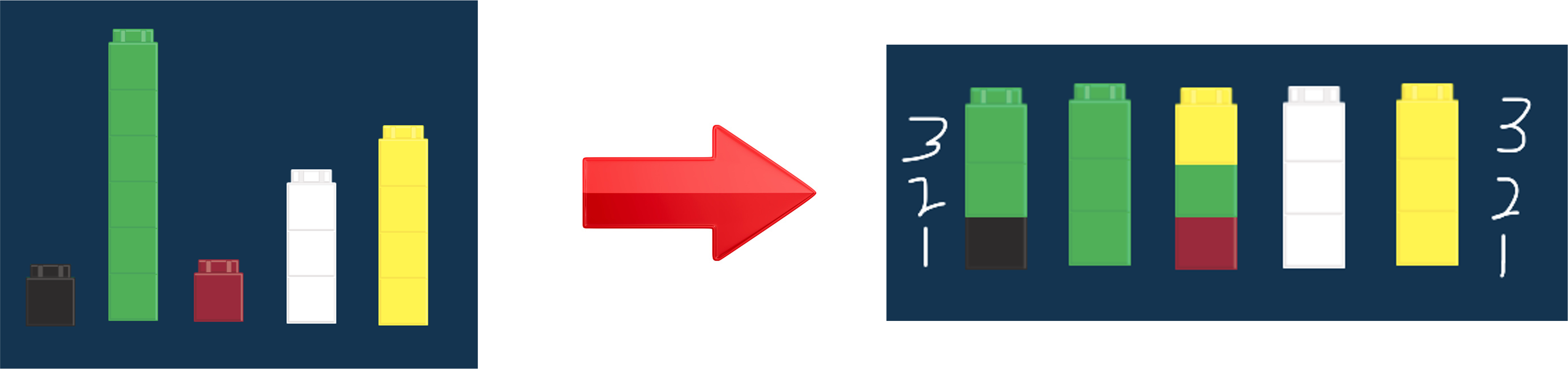
When you think of mean, think “balancing out”
The mean is about equal redistribution. For example, if you took everyone’s wealth and redistributed it so everyone had an equal amount of wealth, that amount of wealth would be the mean.

Calculating the Mean
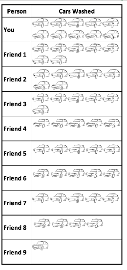
Let’s say you and 9 of your friends were hosting a car wash. Some cars are dirtier than others, some of you are more efficient than others, etc. You don’t all end up washing the same number of cars.

You worked your butt off and washed 10 cars. 2 of your friends washed 7 cars. 1 of your friends washed 6 cars. 4 of your friends washed 5 cars. 1 of your friends washed 4 cars. And 1 of your friends only washed 1 car.
What is the average number of cars washed?
Well, we know you didn’t wash a typical amount of cars among your friend group!
One way to measure this is the median. The median number of cars washed per person was 5 cars.
1 4 5 5 5 5 6 7 7 10 (Those are the number of cars washed in order. There are two middle numbers, both 5. Their midpoint or mean is 5.)
Another is the mean.
In total, you and your friends washed 55 cars.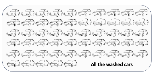
How many cars would each of you needed to wash to each wash the same number of cars? There were 10 of you. I can divide 55 cars up into 10 even groups. 55 ÷ 10 = 5.5. So each of you would have had to wash 5.5 cars. The mean is 5.5, another measure of the average number of cars washed per person.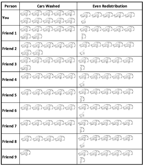
How do I interpret the mean?
On average, each person washed 5 ½ cars. If you balance out the number of cars washed by each person, each person would have 5 ½ cars.
Comparing the mean and median: Is the average 5 or 5.5?
While the mean and median are both averages, they did not give you the exact same answer. This is because the mean took into account all the cars washed and redistributed them, while the median looked for the middle number of cars washed. You washed a lot of cars, which brought the mean up, since all 10 of those cars were included in the total number of cars washed. But whether you had washed 5 or 50 cars, the median would still be 5, as it did not change the number of cars washed by your friends who washed the middle number of cars. Means are influenced by extreme values and outliers, while medians are not.
Mean Calculation
Mean = total Sum of all values ÷ number of items/cases
Sometimes you will see the formula written out with symbols, like this:
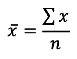 .
. 
Remember that x̄ is the sample mean. Σ, the Greek capital letter Sigma, means sum of. n is the sample size (number of cases). So this formula tells you that you find the sum of the values of all the cases and divided it by the number of cases.
Finding the mean with SPSS:
1. You can find the mean when you run frequencies like you were doing for the range and five point summary.
Menu:
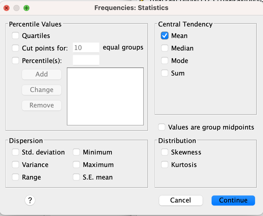
In SPSS, go to Analyze → Descriptive Statistics → Frequencies.
Click on the Statistics button to the right. Then check the box for mean in the upper right of the statistics window and click Continue.
Syntax:
*Include MEAN on the STATISTICS line to include a calculation of mean.
FREQUENCIES VARIABLES=VariableName
/FORMAT=NOTABLE
/STATISTICS=MEAN
/ORDER=ANALYSIS.
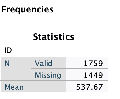
Output:
The row labeled mean gives you the range (e.g., here it is 537.67)
2. You can find the mean with Examine/Explore.
Menu:
Go to Analyze → Descriptive Statistics → Explore. Put your variable into the Dependent List window/box. At the bottom where it says “Display,” make sure you either have “Both” or “Statistics” checked (Plots will only give you graphs/figures).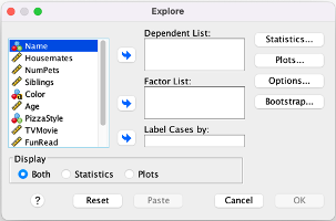
Click OK to run the Explore command.
Syntax:
*This will generate the mean along with other statistics and plots.
EXAMINE VARIABLES=VariableName
/PLOT BOXPLOT HISTOGRAM
/PERCENTILES(25,50,75) HAVERAGE
/STATISTICS DESCRIPTIVES
/CINTERVAL 95
/MISSING LISTWISE
/NOTOTAL.
Levels of Measurement
Caution
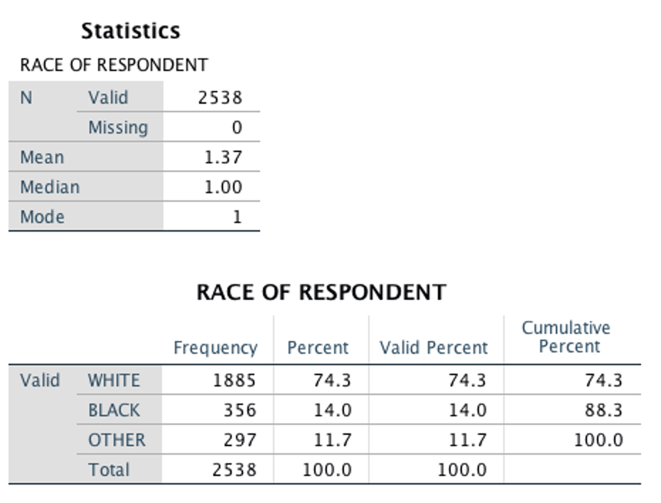
Nominal-level variables do not have interpretable means! (What would be a mean of people’s names? The numbers assigned are arbitrary.) For nominal-level variables only the mode has meaning.
Example: In the SPSS output below, SPSS calculated a mean for respondent race. However, a mean of 1.37 does not have any actual meaning. The mode of 1 means that the value coded as 1 (in this case, White) was the most common/frequent response. That means that (in this sample) there were more white people than black people, and more white people than people of other races.
Indicator-level variables do have an interpretable mean, but with a different interpretation. For indicator variables, the mean is the proportion of respondents with the value coded as 1. An example below elaborates on this.
Statistics in Action: Pay gaps (ratio)